OpenIntroOrg Regression Intercept and Slope Calculation (+more) (Casio fx-9750GII)

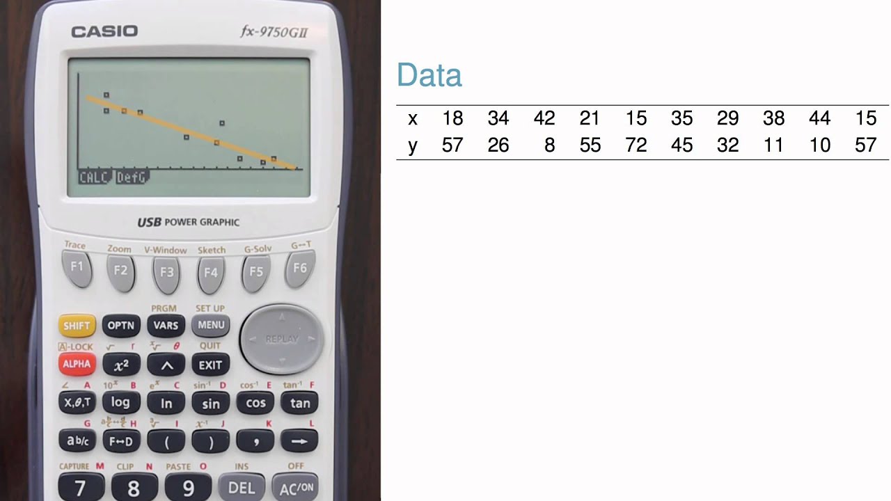
Calculate the y-intercept, slope, correlation, and R-squared of a regression line on a Casio 9750 graphing calculator ( http://amzn.to/1AVxr78).

For more free statistics resources, visit http://www.openintro.org.

Also, check out our free intro statistics textbooks at http://www.openintro.org/stat/textboo...

- - -

Approximate script:

I'm going to cover how to enter data and get a regression line summary using a Casio 9750 graphing calculator, and I'm going to do this in three stages: first enter the data, then look at a graph of the data, and finally fit a regression line.

1. Just like with other statistics calculations, I'll start by going to the STAT section by hitting Menu and then navigating over to Stat.

2. Next, I'll enter the data into two lists. Here I'll use List 1 and List 2, but you can use any two lists you want. However, I'll first need to delete the data that's already in the list, which I can do one observation at a time, or if I arrow over with F6 and choose the delete all option. With that, I'm ready to enter my sample data set, which has 10 observations. It's really important to enter the data in the exact same order in each list.

3. Before I calculate the regression line, it's a good idea to look at the plot. I can do this by navigating to Graph, then set the graph parameters. Here I'm using graph 1, which will be shown as a scatterplot using Lists 1 and 2. If I needed to change a list number, I'd go to the list, hit F1, then enter the proper list number. I find it easier to always use Lists 1 and 2 so I don't need to update this setting every time. But if you do occasionally use other lists, verify the proper lists are set. Now I can exit out and show graph 1. A downward trend is evident in the data, so I should expect to see a negative slope when fitting the line. The trend also looks reasonably stable, and there are no outliers that would be a cause for concern.

4. Alright, now that I've checked that the data look reasonable for a regression line, I'll exit out, go to CALC, then SET, and I'll specify the regression context. For example, I need to make sure the proper lists are set, just like I did when graphing. Exiting back out to the previous screen, I'm finally ready to compute the regression line. To do so, I choose REG for regression line, X for a linear regression line, and I prefer the form a + bx, so I'll choose that option.

The regression output shows
- the form of the equation,
- the y-intercept of the best-fit line,
- the slope of the best-fit line,
- the correlation,
- the R-squared value, and
- the mean squared error of the residuals.

This last statistic usually isn't discussed in introductory statistics courses. The final equation of the line is y = 93.71 - 1.94 * x. Notice the negative slope, which made sense with the scatterplot I examined earlier. Here's a plot of the data with the regression line shown, which was created using a statistical software called R.

In the next video, I'll cover how to perform a t-test to evaluate whether there is strong evidence that the slope of the line is different than zero.

If you liked this video, give it a thumbs up below and subscribe. Thanks for watching.

Regression Intercept and Slope Calculation (+more) (Casio fx-9750GII)
485 Likes	485 Dislikes
48,843 views views	5,580 followers
Education	Upload TimePublished on 19 Jul 2015